Liebmann - (still unfinished) software to make charged particle optics computations.

About program

Liebmann software is intended to make computations of electron / ion optical systems.
Currently, it allows the determination of electrostatic field distributions in a vacuum. It solves problems involving electrodes (i.e., points at a fixed potential) and a vacuum. No dielectrics.

Why calculate the electric field?

In charged particle optics, one of the issues is determining the distributions of electric and magnetic fields. If we know the field distribution well, then we can determine the paths of electrons in such a field. This can be used in the design of scientific or industrial devices.

Electrostatic field generated by electrodes of any shape

In school, we usually learn about the electrostatic field in the form of Coulomb's law and Gauss's law. Coulomb's law allows us to determine the distribution of the electrostatic field generated by point charges. However, there are issues that go beyond such theory. How to determine the electrostatic field when, for example, the electrodes have irregular shapes and cannot be treated as points? We know that the surface of a metal electrode has a constant potential. We need to determine the distribution of the field in the vicinity of the electrodes. Some electrode systems can be described using advanced mathematical methods. Fortunately, mathematical scientists have also invented numerical methods that can be used for calculations with any shape of electrodes. This page is about such a method. The electrostatic field is described by the Laplace equation. It is solved using the Liebmann relaxation method.

Laplace equation

Liebmann software can solve Laplace equation.

This is partial differential equation, which describes electrostatic field in vacuum. For our purposes, we can assume that we have metal electrodes placed in a vacuum. It is assumed that the surface of the metal electrode has a fixed potential, set, for example, by means of a power supply. In the environment of the electrodes with fixed potentials, there is an electrostatic field, the distribution of which we want to determine. We want do determine electrostatic potential in all mesh points, which represent vacuum.

Laplace equation in one-dimensional form has form:

After integrating side by side, we obtain the solution - a one-dimensional, uniform electrostatic field.

After another integrating, we obtain solution of potential V(x) - linear function.

Laplace equation in 2D coordinates X-Y (planar) takes form:

Laplace equation in 3D coordinates X-Y-Z takes form:

Laplace equation in 2D coordinates Z-R (cylindrical symmetry) takes form:

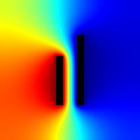
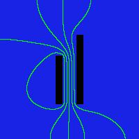
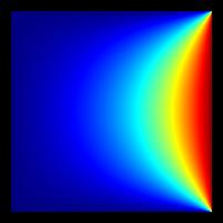
Example - Laplace equation (2D, X-Y) for the problem of two plates of different lengths

The following example presents a non-standard problem. It is a two-dimensional (X-Y) problem. The figure on the left shows the numerical mesh used in the calculations. It contains two plane-parallel plates in a vacuum. However, they have different lengths. The mesh has 200 rows and 200 columns. The green electrode has a potential of -1.0 [V]. The red electrode has a potential of +1.0 [V]. The white points surrounding the plates represent the vacuum. We want to determine the potential distribution at the points representing the vacuum.

This can be calculated, for example, using the relaxation method, which is possible with the Liebmann program. The middle image shows the calculation result, i.e., mapping the calculated potential to colours. Jet mapping algorithm (described in the documentation). The right image shows the equipotential lines of the calculated potential. A detailed description of the problem is available in the gallery (problem no. 9).

Pictures on this site have 2 pixels wide frames.

Relaxation method

The Liebmann program uses the relaxation method (successive approximations). This method is called the Liebmann relaxation method. The goal is to determine the electric potential distribution at points representing the vacuum. The relaxation method involves performing a relaxation procedure for each point representing the vacuum. For a point within a mesh, this may seem simple (in 2D X-Y geometry) (adding the potentials of the four neighbors of a given node to the left, right, top, and bottom, and then dividing the sum by 4). The relaxation formulas depend on the type of coordinate system and the position on the mesh. In 2D cylindrical coordinates (ZR), dependencies appear on the distance of the point from the Oz axis; on the Oz axis, some derivatives require non-trivial procedures.

After each such procedure, we check how much the new potential value has changed compared to the value previously stored in our node. This allows us to determine the largest potential change across the entire numerical mesh. When subsequent applications of the relaxation procedure to the mesh do not result in significant changes to the desired potential distribution, the calculations are stopped, and the potential distribution on the mesh is treated as the newly found solution. The obtained results are saved to the output files.

Technical details

Liebmann software is based on robust FLOSS tools (ANSI C language, gcc compiler).
Liebmann is being developed on 2 environments:

• Linux Mint - (gcc, xed, texlive, netpbm)
• MS Windows(TM) - gcc (MinGW-w64, MSYS2, UCRT64), Notepad++, MiKTeX, Faststone Image Viewer)

At the moment Liebmann consists of modules:

• Module (relax_xy) contains algorithms to calculate distribution of electrostatic potential in 2D flat coordinates (X-Y).
• Module (mesh_xy) contains functions to support numerical meshes (eg. setting potentials of nodes, writing mesh to file .DAT, .BMP, .PPM)
• Module (anls_xy) contains algorithms to analyze output data (eg. determination of equipotential lines).
• Module (relax_rz) calculates electrostatic field in 2D cylindrical coordiantes (Z-R).
• Module (colormap) does mapping of potential and other calculated values to colours.
• Files (demo_xy_problems) contains functions to define problems to solve (10 problems per file). Definition of problems (shape of electrodes) uses elements of geometry - rectangles, circles and ellipses.

These modules are written in ANSI C language. Only writing to BMP file requires stdint.h file from C99 standard.

At the moment defining of problem to solve is defined "directly in source code". Only functions, which set meshes for each problem to solve have been moved to separate files. They are places in demo_xy_problem files (10 functions per file). Defining problems (entering electrode shapes) uses elements of analytical geometry - rectangles, circles, ellipses, polar coordinates.

DEMO executables

Liebmann algorithms are used in two executables DEMO_*. These programs are such as technology demonstration of Liebmann possibilities.

• Program DEMO_XY determines electrostatic field for several dozen of electrostatic problems, which are have been defined "in program's code".
• Program DEMO_ZR determines electrostatic field of 3 electrode electrostatic unipotential "einzel" lens. At the moment it has not been checked carefully.

Running DEMO program

1. First unzip Liebmann project archive to known directory.
2. Source code files are situated in directory: source_code_ansi_c.

Names of executable fiels are:

• DEMO_XY.exe (version for MS Windows (TM) operating system).
• DEMO_XY.run (version for Linux operating system).

Microprecessor architecture

• Exacutables has been compiled by default for architecture x86_64.
• If we want to change architecture, we must recompile project with changed compiler options (flag march).

Text terminal under MS Windows(TM)

In Windows OS we can run compiled program using console cmd.exe

1. Run cmd.exe in Windows menu (text terminal).
2. Change directory to directory with DEMO executables.
3. Now we can run program (for example problem No.1) - use command: DEMO.XY.exe 1
4. If program executes successfully, results are written to outputs catalogs.
5. We must remember, that only catalog outputs_xy_jpg is extraordinary. In Linux OS this catalog is written during serial conversion files from standard PPM do JPG.
6. To watch PPM files additional image viewer is needed, for example Fast Stone Image Viewer (TM).

Option with MSYS2 environment. Liebmann project id being developed in MSYS2, UCRT64 environment. This environment uses bash shell.

1. We run MSYS2 UCRT64
2. On my computer project is situated in directory (for user ADS) C:\msys64\home\ADS
3. We enter catalog with executables DEMO (cd Liebmann_project/source_code_ansi_c).
4. We can run program (for example problem No.1) - we use command: ./DEMO.XY.exe 1
5. If program executes successfully, results are written to outputs catalogs.
6. We must remember, that only catalog outputs_xy_jpg is extraordinary. In Linux OS this catalog is written during serial conversion files from standard PPM do JPG.
7. To watch PPM files additional image viewer is needed, for example Fast Stone Image Viewer (TM).

Under MSYS2 UCRT64 environment we can also compile project. We need gcc package for appropriate version of environment. I use command (for pacman package manager):

pacman -S mingw-w64-ucrt-x86_64-gcc

Windows should see gcc compiler, so we need to add another path to Path System Enviromnent (path to tools for MSYS2).

C:\msys64\ucrt\bin

When we have gcc under MSYS2 UCRT64 enviromnent, we can compile project by script build_demo_xy_mingw_ucrt.

Text terminal under Linux

In Linux we run text console.

1. Unzip project.
2. We enter to unzipped project.
3. Source files and executables are in directory: source_code_ansi_c
4. Some files must have privilegdes to be executed: 2 commands: chmod +x *.run , chmod +x *.bash
5. We can run program (for example problem No. 1) - we use command: ./DEMO.XY.run 1
6. If program executes successfully, results are written to outputs catalogs.
7. We must remember, that catalog outputs_xy_jpg is extraordinary. We can convert all files from format PPM to JPG using script demo_xy_convert_to_jpg.bash. We need to install package netpbm.
8. To watching picture standard picture viewer should be sufficient.

Compilation

Each program has its own compiling script. Their names are "build" and appropriate rest of name.

DEMO_XY
Linux      - build_demo_xy_linux.bash
MS Windows - build_demo_xy_mingw_ucrt.bash

DEMO_ZR
Linux       - build_demo_zr_linux.bash
MS Windows  - build_demo_zr_mingw_ucrt.bash

Script build runs compiler gcc (Linux) or MinGW (Windows) with many addidtional flags (based on GNU GSL library). Under Linux each script must have permission to be run (command chmod +x *.bash).

Results

Computation results are written (or not, if failure) to "outputs" catalog for each program. Graphic files have format .PBM and text files have .dat extension. Under Linux .PBM files should be easily displayed by default file manager. Under Windows you can use additional image viewer (I have tested Fast Stone Image Viewer).

• Computation results are written (or not, if failure) to directories "outputs" for appropriate program and format.
• Graphic files have formats .BMP and .PPM
• Text files have extension .dat.
• Under Linux OS .PPM files could be able to be opened by typical picture viewer.
• Under Linux OS all the .PPM files can be converted to .JPG standard and moved to other catalog by script demo_xy_convert and package netpbm (ppmtojpeg program).
• Under Windows OS user can watch .BMP files. Additional picture browser can be used to browse .PPM files (I have tested with Fast Stone Image Viewer).

Licence

Liebmann software is available under free license GPL v.3.0+ (version 3.0 or any later).

Galleries

Example - map of electrostatic potential of plane vacuum diode with lateral plates at the cathode potential.

• Link to the whole catalogue of galleries.

Download

• files with project (ANSI C + bash + binaries) (20260414)
• the whole documentation (relaxation schemes, LaTeX files) (20250911)
• truncated binary version for MS Windows x86_64 (20260414)
• documentation (relaxation scheme XY) (20250313)
• documentation (relaxation scheme ZR) (20241213)
• documentation (colormap) (20240718)

Older versions

I have removed older versions because they had significant bugs. This is a good download if your network services block .zip files containing .exe files.

• the whole project Liebmann (20250824)

You Tube

• (Polish version) Pole elektrostatyczne w otoczeniu dwóch płytek o różnej długości. Obliczenia numeryczne (wersja 3).

Info about project

• Project is being developed in "free time" by Marcin Kulbaka.
• Project has started in 2020 (during COVID 19 pandemia).
• Project is a kind of "continuation" of research started during MSc studies (master's thesis "electron optical systems").
• The master's degree was being pursued at predecesor of current Department of Surface and Nanostructures Physics (Institute of Physics, UMCS, Lublin).

References

Charged particle optics

1. Pierre Grivet, "Electron Optics", 2nd. edition, Part 1 Optics, Pergamon Press 1972
2. Pierre Grivet, "Electron Optics", Pergamon Press 1965
3. James R.Nagel, "Solving the Generalized Poisson Equation Using the Finite-Difference Method (FDM)"
4. Albert Septier, "Focusing of Charged Particles", Volume I, Academic Press 1967.
5. Bohdan Paszkowski, "Optyka Elektronowa", Wydanie II, Wydawnictwa Naukowo - Techniczne, Warszawa 1965 (Polish edition)
6. Bohdan Paszkowski, "Electron Optics", Iliffe Books Ltd. 1968 (English edition)
7. DWO Heddle, "Electrostatic Lens Systems", IOP Publishing, Bristol and Philadelphia 2000
8. Jon Orloff, "Handbook od Charged Particle Optics", 2nd edition, CRC Press 2009
9. Albert Septier, "Applied Charged Particle Optics", Part A, Academic Press 1980

Programming and numerical methods

1. Introduction to algorithmization and programming, lecture and exercises, UMCS 2003
2. Bogdan Buczek, "Algorytmy. Ćwiczenia." Helion 2008
3. Algorithmization and programming, lecture and exercises, UMCS 2007
4. Niklaus Wirth, "Algorytmy + struktury danych = programy", wydanie szóste, Wydawnictwo Naukowo - Techniczne, Warszawa 2002 (Polish edition)
5. Niklaus Wirth, "Algorithms + data structures = programs", first edition, Prentice Hall 1976 (English edition).
6. Programming in C language, lecture and exercises, UMCS, 2007
7. Donald Alcook, "Illustrating C", Cambridge University Press (1994).
8. Numerical methods, lecture and exercises, UMCS 2006
9. MATLAB - environment for numerical calculations (it has got wide documentation) link
10. SIMION - charged particle optics simulation software link
11. IBSimu - free ion beam simulator (with space charge efects) (GNU GPL license) link
12. Stephen Prata, "C Primer Plus", Addison - Wesley (English edition)
13. Stephen Prata, "Szkoła programowania. Język C.", Helion, Gliwice(Polish edition)
14. Kyle Loudon, "Mastering Algorithms with C", 3rd Edition, O'Reilly Media (1999)
15. Kyle Loudon, "Algorytmy w C, Helion Gliwice (Polish edition)
16. Richard Reese, "Understanding and using C pointers", O'Reilly Media (English edition)
17. Richard Reese, "Wskaźniki w języku C. Przewodnik", Helion Gliwice (2014) (Polish edition)
18. Zed A. Shaw, "Learn C the Hard Way: Practical Exercises on the Computational Subjects You Keep Avoiding (Like C)", Addison - Wesley (English Edition)
19. Zed A. Shaw, "Programowanie w C. Sprytne podejście do trudnych zagadnień, których wolałbyś unikać (takich jak język C)", Helion Gliwice (Polish Edition)
20. Andrew Koenig, "C traps and pitfalls", Addison-Wesley Professional (1989)
21. https://cplusplus.com (for example reference to standard C library, examples) link
22. https://en.wikibooks.org/wiki/C_Programming link
23. https://pl.wikibooks.org/wiki/C link
24. https://stackoverflow.com (np.for example problems with compilation, tutorials etc.) link
25. Andrew Hunt, David Thomas, "Pragmatic Programmer, The: From Journeyman to Master", Addison Wesley 1999 (English edition)
26. Andrew Hunt, David Thomas, "Pragmatyczny programista. Od czeladnika do mistrza.", Helion Gliwice, (Polish edition)
27. B. M. Harwani, "Practical C Programming. Solutions for modern C developers to create efficient and well-structured programs", Packt 2020.
28. Richard F. Gilberg, Behrouz A. Forouzan, "Data Structures: A Pseudocode Approach with C". Second Edition, (C) 2005 Course Technology, a division of Thomson Learning, Inc.
29. Suad Alagic, Michael A. Arbib, "The Design of Well-Structured and Correct Programs", Springer 1978

Writing images directly to graphical files

1. NetPBM file format link
2. BMP file format link
3. OpenGL tutorial: loading BMP files yourself
4. StackOverflow: create-simple-bitmap-in-c-without-external-libraries
5. StackOverflow Creating bitmap using C

Computational geometry

1. Intersection of line two segments (on StackOverflow forum) link
2. Intersection of line segment and circle (on StackOverflow forum) link

Program libraries

1. Program libraries on Linux - HOWTO link
2. Program libraries (DLL) on Microsoft Windows (TM) - Wikipedia link

I would not recommend search publications in "shadow libraries" (violation of copyrights etc.).

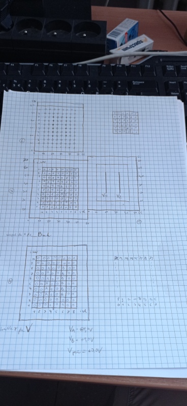
Photos of project realization

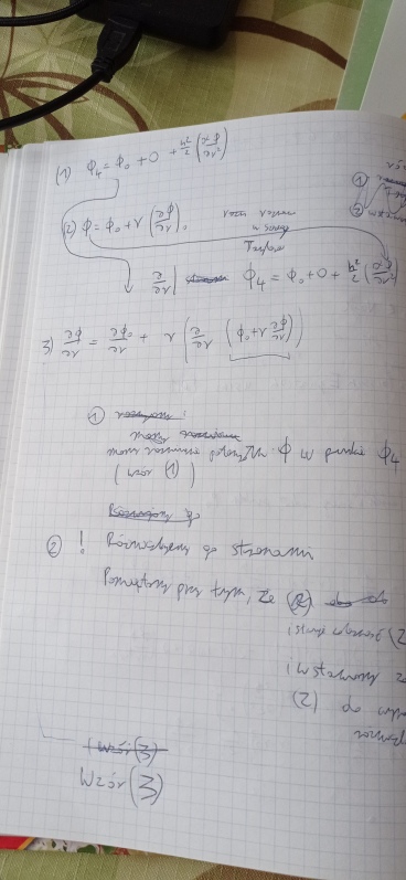
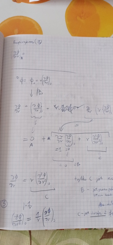
The beginnings were not brillant. In fact I don't know, whether final versions are fully correct. I did my best. The third attempt was probably better.

Early drafts

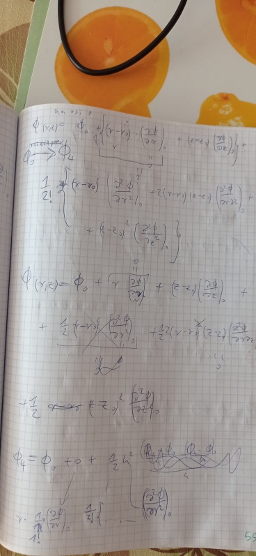
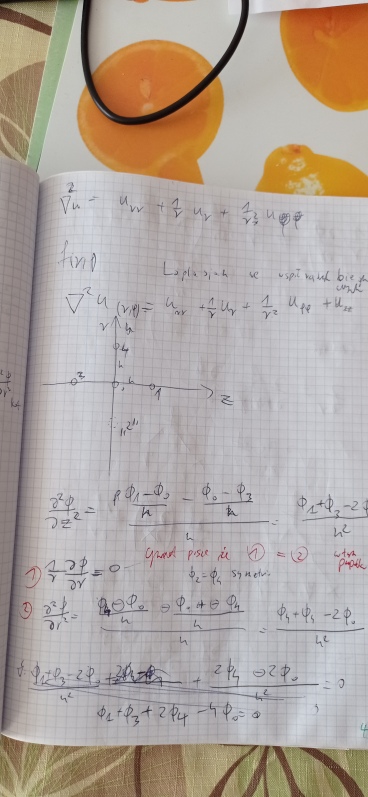
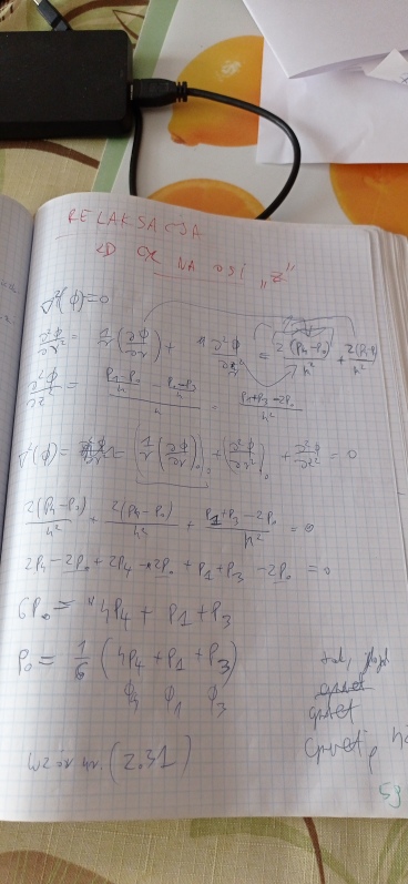
Some time later another versions of theory seemed to have any sense

Final versions for LaTeX

footer

This static site does not use any cookies or gather any data.